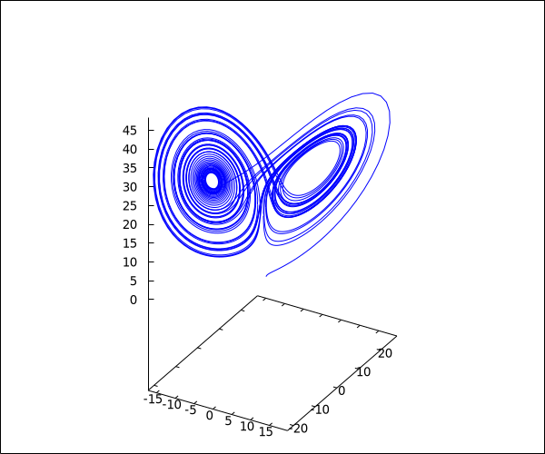
I was reading the Wikipedia page for the famous Lorenz system of differential equations, and saw a nice animated plot of the phase space written in the Julia language. Among the other code examples on that page is a solution for Maxima, which outputs the following when run:

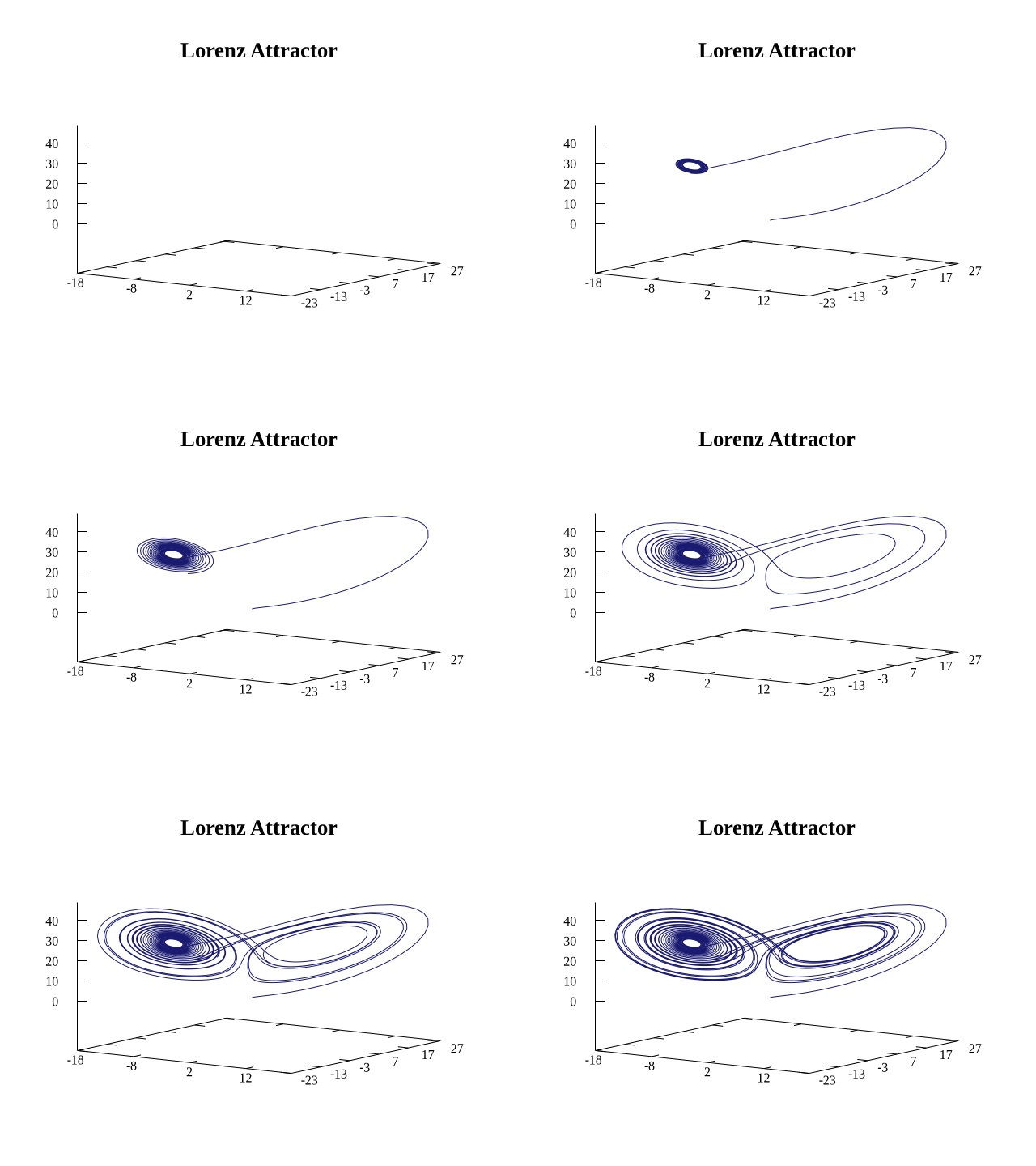
It's not a bad plot, but I thought it could be improved. Here is my version:

Maxima has plotting functions, but these are just an interface to external programs. Maxima mostly relies on gnuplot, an external scientific plotting program (which interestingly has nothing to do with GNU). The built-in functions are easy to use, and the Maxima IDE wxMaxima provides some of its own functions to help. In particular, the use of with_slider_draw3d() makes it easy to create an animated GIF of a plot. At the end of this post, I will provide an alternative solution using only wxMaxima, but we will see that it gives less control over the final output.

Any kind of plot needs to start with a numerical solution to the system of equations. For that, we can use the rk() function, which implements the classic fourth-order Runge-Kutta method.

[sigma, rho, beta]: [10, 28, 8/3]$
eq: [sigma*(y-x), x*(rho-z)-y, x*y-beta*z]$
sol: rk(eq, [x, y, z], [1, 0, 0], [t, 0, 40, 1/100])$

To export the solution data given by rk(), we can load the numericalio package for the write_data() function. Gnuplot expects a data file where each row describes a point, with the columns representing x, y, z (in that order). Putting the data first into a matrix and transposing it is a trick to get that form.

load("numericalio")$
len: length(sol)$
x: makelist(sol[k][2], k, len)$
y: makelist(sol[k][3], k, len)$
z: makelist(sol[k][4], k, len)$
data: transpose(matrix(x,y,z))$
write_data(data,"home/Documents/data_out.dat")$

Now for the gnuplot script "lorenz.gnu". One thing to know about gnuplot is that there are quite a few terminals you can set, and they all affect the type of output you get. Initially, I tried the gif terminal:

set terminal gif animate loop 0

set output 'lorenz_animation.gif'
set title "Lorenz Attractor"

do for [alpha = 1:359] {
set view 75,alpha
splot 'data_out.dat' with lines linecolor "midnight-blue" title ""
}

The output is pretty bad. This won't do at all! But do for could also be used to repeatedly save output files using a different terminal, which could be compiled into an animation. The only problem is how to make gnuplot incrementally plot points so the illusion of motion can be achieved. One way to make gnuplot do this is with the every keyword. For example, plot 'data_out.dat' every ::5::15 will draw points 5 through 15. If instead we use plot 'data_out.dat' every ::1::k, where k is a for loop index, we are in business. Except… my data file has 4,001 rows. Hence, k stepping one at a time will take forever. Luckily gnuplot allows specifying increments in a for loop using [k ​ start:end:increment]=. Increments that are too small will generate an unnecessary number of frames, while making them too large will ruin the playback – after playing around with it, I settled on increments of 16 as an adequate compromise.

There also needs to be some way to vary the name of the output file with each iteration, otherwise gnuplot will only save one file and continue to overwrite it. A classic loop counter variable is an easy way to accomplish that. I don't think I've implemented one since my freshman year course on introductory programming!

set terminal pngcairo size 768, 576 font "Liberation Serif Bold, 20"

stop_run = 4001

i = 1

do for [k = 1:stop_run:16] {
set output sprintf('./Outputs/lorenz_gnuplot_%d.png',i)
i = i + 1
set title "Lorenz Attractor"
set tics font "Liberation Serif, 12"
set view 75,35
splot 'data_out.dat' every ::1::k with lines linecolor "midnight-blue" title ""
unset output
}

One last improvement to the script makes use of the stats command gnuplot provides to calculate bounds for the axes. If you don't put those in somehow, gnuplot will autoscale the axes but I didn't like the way this looked when animated (YMMV). stats is a brilliant feature, but it only works on two columns at a time so the results have to be captured in custom variables.

set terminal pngcairo size 768, 576 font "Liberation Serif Bold, 20"

stats 'data_out.dat' using 1:2
x_lower = floor(STATS_min_x)
x_upper = ceil(STATS_max_x)

y_lower = floor(STATS_min_y)
y_upper = ceil(STATS_max_y)

stats 'data_out.dat' using 3
z_lower = floor(STATS_min)
z_upper = ceil(STATS_max)

stop_run = STATS_records

i = 1

do for [k = 1:stop_run:16] {
set output sprintf('./Outputs/lorenz_gnuplot_%d.png',i)
i = i + 1
set title "Lorenz Attractor"
set tics font "Liberation Serif, 12"
set xtics autofreq x_lower, 10, x_upper offset graph 0.09, -0.09
set ytics autofreq y_lower, 10, y_upper offset graph 0.05, -0.08
set ztics autofreq 0, 10, z_upper
set xrange [x_lower:x_upper]
set yrange [y_lower:y_upper]
set zrange [z_lower:z_upper]
set view 75,35
splot 'data_out.dat' every ::1::k with lines linecolor "midnight-blue" title ""
unset output
}

Executing in the command line, gnuplot takes a few seconds to chew through this. To generate the animation, you can use the convert command provided by ImageMagick. This step is probably the slowest, especially if you generate a gif file.

The settings I settled on are:

convert -delay 5 -loop 0 -dispose Background lorenz_gnuplot_{1..251}.png lorenz.webp

You have to change 251 to the number of frames generated by gnuplot, which depends on how the simulation is set up and the increment size in the do for loop.

Another way, run in wxMaxima:

kill(x,y,z)$
[sigma, rho, beta]: [10, 28, 8/3]$
eq: [sigma*(y-x), x*(rho-z)-y, x*y-beta*z]$
sol: rk(eq, [x, y, z], [1, 0, 0], [t, 0, 50, 1/80])$
len: length(sol)$
x: makelist(sol[k][2], k, len)$
y: makelist(sol[k][3], k, len)$
z: makelist(sol[k][4], k, len)$
L: round_bounds(bounds(x,y,z))$
wxanimate_framerate:20$
wxplot_size:[840,700]$
with_slider_draw3d(
    k,makelist(i,i,1,len,20),
    title = "Lorenz Attractor",
    points_joined=true,
    color = midnight_blue,
    point_type = -1,
    xrange = [L[1][1],L[1][2]], yrange = [L[2][1],L[2][2]], zrange = [0,L[3][2]],
    points(firstn(x,k),firstn(y,k),firstn(z,k)),
    view = [75,35],
    axis_3d = true
)$

Where round_bounds() and bounds() are homemade helper functions:

bounds(x,y,z) := (
    makelist(
        [apply(min, l),apply(max, l)],l,[x,y,z]
    )
)$

round_bounds(L) := (
    makelist(
        [floor(L[i][1]), ceiling(L[i][2])], i, 1, 3
    )
)$

The wxMaxima approach also works well, but as far as I know there is no control over the plot title offset as in native gnuplot, and you can only set one font size for the whole plot.

Tags: math, maxima, programming, gnuplot.